
[cea-b-02] PV panels and where to place them 1: value for money?
Want the highest possible PV electricity yield? To achieve this, a simple method is to apply PV panels onto every inch of the building envelope. However, obviously it is not always this simple. This CEA Lesson provides you a method to identify the building envelope surfaces for PV installations using CEA.
This CEA Lesson is under the BIPV Design Module required by the Designer Track.
The design proposal below titled MAISON DE LA SANTÉ BIEL presents an interesting award-winning design using BIPV. The building is elegantly enveloped by solar façade that offers energy generation. Almost the entire building volume is covered with such solar materials, based on the limited images we have found. However, does it make sense to cover “everywhere“ with PV economically?
In the next section of BIPV metrics, we are introducing two metrics measuring the BIPV efficiency, in terms of value-for-money?

1. Before all, what-is-needed?
Before we proceed, we need to make sure that we have the following item(s) done or in-place.
CEA Lesson prerequisites
Do follow CEA Lesson [cea-v-01] first
Data
Check Folder: {Your Project} > {Your Scenario} > outputs > data > potentials > solar
Make sure such a .csv CEA file exist: PV_total_buildings; if not, execute CEA Simulation: Energy potentials > Photovoltaic panels
2. BIPV metrics
In this CEA Lesson, we introduce two BIPV metrics to assess value-for-money and guide BIPV design. They are unit cost [USD/kWh] and annual solar insolation [kWh/m2/yr]. Their details are as follows.
unit cost
A BIPV system’s unit cost is the price incurred to produce and store of one unit of PV electricity. The equations used to calculate unit cost [USD/kWh] of a building or a district (i.e. a cluster of buildings) are:

, where we use approximately 10% of the annualized capital cost for O&M cost; annual PV electricity yield equals Column named ‘E_PV_gen_kWh’ in the .csv CEA File named ‘PV_total_buildings’; and

, where total capital cost equals approximately 200 USD/m2 (note: you may want to research on this number in your own economy) multiplied by the installed area of PV to be found under Column named ‘Area_PV_m2‘ in the .csv CEA File named ‘PV_total_buildings’; n equals approximately 20 years of PV life time; and i equals to the interest rate at 5% (note: you may want to adjust this number for your own economy).
annual solar insolation
Annual solar insolation is the amount of solar energy incident on a specified area over a year. In CEA simulations, annual solar insolation is used a user-defined threshold to determine where to place the PV panels on the building envelopes. Users can define the annual solar insolation under: Energy potentials > Photovoltaic panels > annual-radiation-threshold (Fig.cea-b-02-03).

Fig.cea-b-02-03 presents the input interface of the CEA Dashboard for annual solar insolation. In this example, CEA will only apply PV panels to CEA sub-surfaces of building envelopes that have an annual solar insolation of 800 kWh/m2/yr or above.
Please be noted that the default 800 kWh/m2/year threshold is a quick-n’-easy rules-of-thumb we use. In this CEA Lesson, we want you to know how to use BIPV’s unit cost to determine this threshold.
In Section Follow-next-steps, we are walking you through how to use the two metrics to place PV panels on building envelopes in terms of value-for-money.
3. Follow-next-steps
Follow closely the steps listed below. We use the same case study in CEA Lesson [cea-v-01].
Step 1. Iterate CEA photovoltaic panels simulations.
Execute CEA photovoltaic panels simulations for 5 times with the annual-radiation-threshold (Fig.cea-b-02-03) set at 0, 200, 400, 600, and 800;
Upon completion of each iteration, record Column named ‘E_PV_gen_kWh’ in the .csv CEA File named ‘PV_total_buildings’ for your target building(s);
Also, record Column named ‘Area_PV_m2‘ in the .csv CEA File named ‘PV_total_buildings’ for your target building(s).
Step 2. Calculate the BIPV metrics.
Follow the equations in the previous section and calculate the BIPV unit cost for each iteration;
Record your results using the format of table below.

Step 3. Plot the results and make the decision.
As our example below, plot the annual solar insolation on Axis-X and the corresponding BIPV’s unit cost on Axis-Y;
Determine the threshold of annual solar insolation for PV deployment.
For our example, it makes not much sense to apply everywhere on the building envelope with PV panels (i.e. setting the annual solar insolation threshold at 0 kWh/m2/yr). Iteration #3 costs almost three times than #5 while having less than 50% more PV electricity yield, hence as a compromise, we may land on the answer of 600 kWh/m2/year as the annual solar insolation threshold. We can imagine, you may reach a completely different answer as your building may be located in a different location, have more shadings from the surrounding buildings and be restricted by a tighter budget.
We use aggregated results for the entire building while CEA results differentiate Area_PV_m2 and E_PV_gen_kWh by (east, south, west, north) façade and rooftop. You may want to evaluate the these surfaces separately when deciding on the PV deployment.
Do share your results and your reasoning with us on the CEA Forum : )
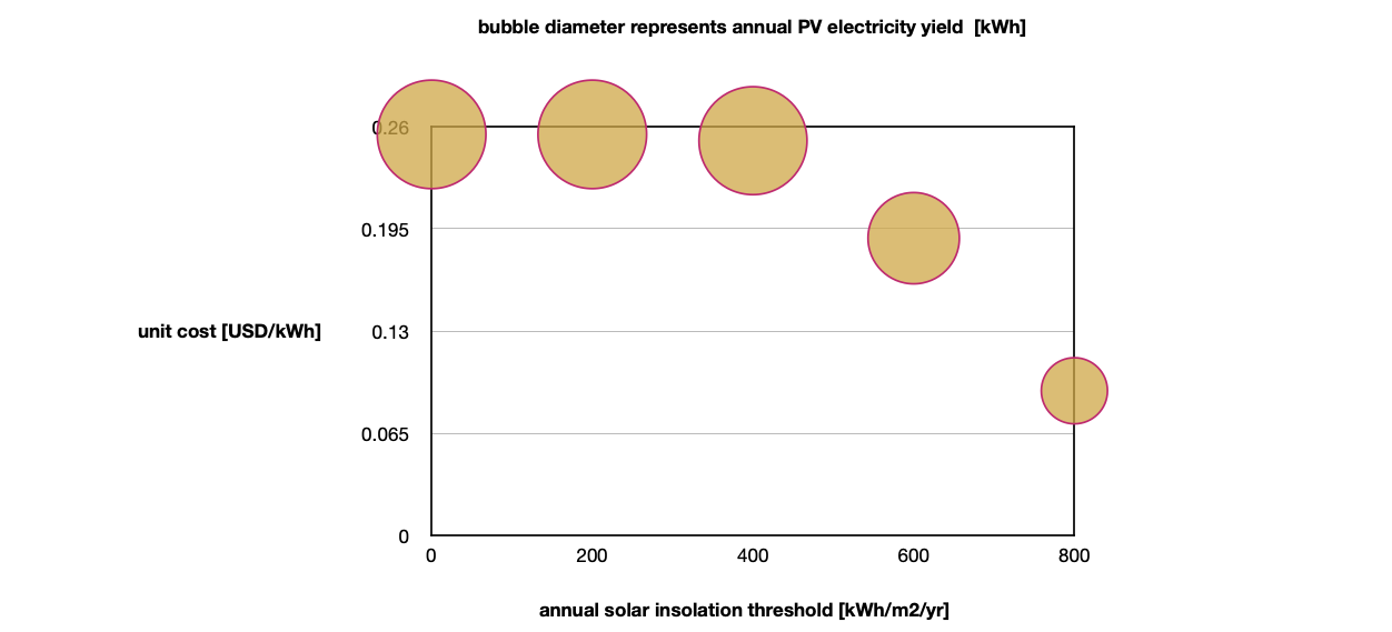
Fig.cea-b-02-04 plots the results for the five iteration of CEA (photovoltaic panels) simulations.
4. How-to-use-it?
Now that we have identified 600 kWh/m2/yr as the threshold of annual solar insolation for PV deployment, what is the next step?
We use the visualization work created following the steps in CEA Lesson [cea-v-01]. Fig.cea-b-02-05 presents a method to visualize the CEA sensors on the unfolded building envelopes. Fig.cea-b-02-06 presents solar insolation zones identified based on the CEA simulation and visualization. Any further BIPV design can be carried out based on these zones.

Fig.cea-b-02-05 is adapted from the work of Natalie Sandelli, Erika Sieweke, and Adam Achtenberg.
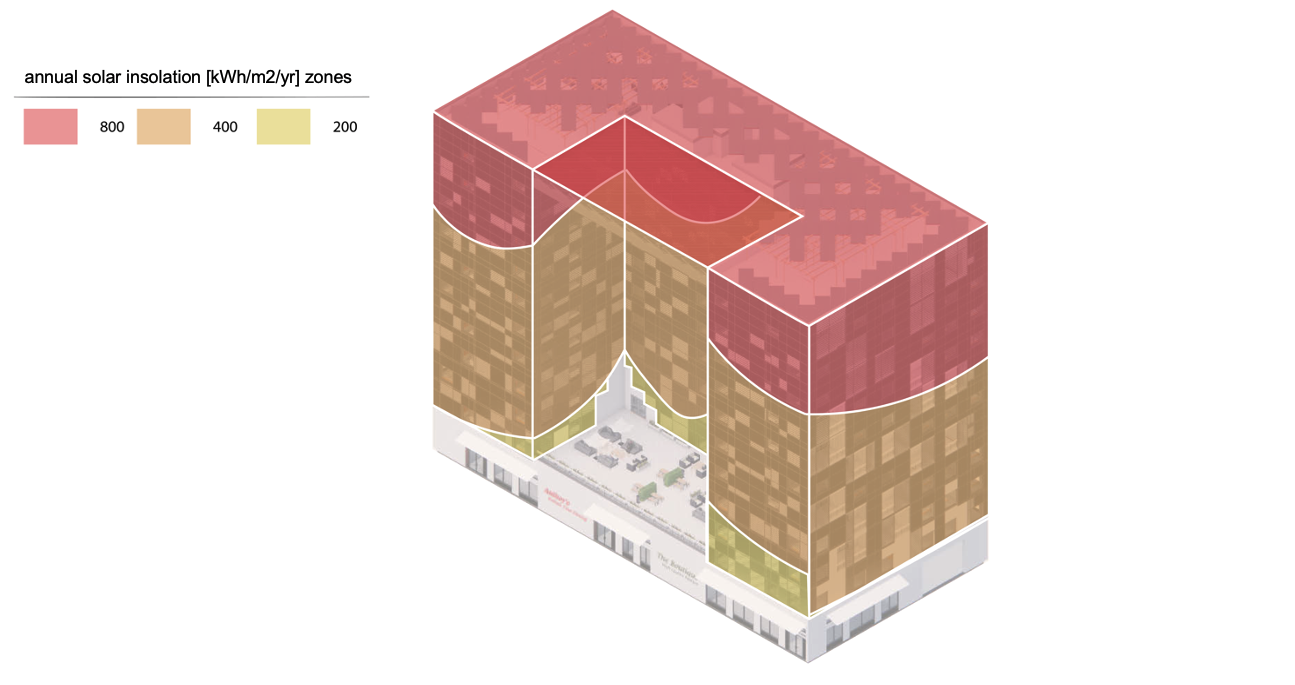
Fig.cea-b-02-06 is adapted from the work of Natalie Sandelli, Erika Sieweke, and Adam Achtenberg.
We believe after this CEA Lesson, you are having your first taste how to use CEA simulation results to guide your BIPV urban or building design. As you can well imagine, cost would not be the only dimension impacting the decision. Hence, in the upcoming CEA Lessons in this module, we will be introducing more dimensions of BIPV metrics into the BIPV design-decision-making processes.
You may now proceed to CEA Lesson [cea-b-03], where more BIPV metrics are introduced for BIPV efficiency assessment and BIPV design.
5. One-step-further
The method we have introduced above is rather simplified as in reality modeling the cost of BIPV also need to consider the hardware costs of non-PV module systems and soft costs including design, construction & installation, permit, inspection, and disposal.
Using cost a metric, the process of PV deployment is beyond being merely spatial (i.e. where to place them). The process also has a temporal dimension (i.e. when to place them). For example, the capital costs of PV have decreased over the past years and there is a continuing trend as such. Hence, deploying PV panels on certain part of the building envelope may not economically make sense in the Year 2023 until Year 2030. As an urban designer or architect, you may want to take the temporal dimension into consideration, come up with a phasing strategy, and keep your design flexible and adaptable.
6. Questions?
Encountering difficulties or having questions ? Proceed to the CEA Forum to post your questions. Your questions may be universal and can benefit other CEA users. Please include the Lesson Code [cea-b-02] when posting your question.