[cea-v-01] Visualise CEA solar simulation results on building envelopes

Want to visualise your CEA solar simulation results on 3D building envelopes like the one below? This lesson guides you through a method to visualise CEA Solar simulation results on building envelopes using Rhino and Grasshopper.

This CEA Lesson is under the Visualisation Module required by the Designer Track and is Optional for the Engineer Track.

** Currently, the content in this CEA Lesson is updated for CEA v3.32.0 or before.

Fig.cea-v-01-01 visualises the CEA-simulated solar insolation results on the building envelope of a residential building in Clementi, Singapore.

Before all, what-is-needed?

Before we proceed, we need to make sure that we have the following items in place.

Data

• Check Folder: {Your Project} > {Your Scenario} > outputs > data > solar-radiation

• Make sure such .csv files exist: {Building Name}_geometry and {Building Name}_radiation

• Check Folder: {Your Project} > {Your Scenario} > inputs > building-geometry

• Make sure such a .shp file exists: zone

Tools

• Make sure you have Rhino 6 or a later version installed.

• Make sure you have a plug-in for Grasshopper that can read .csv files installed. In this tutorial, we use LUNCHBOX (by Nathan Miller) as an example.

Follow-next-steps

Now, follow closely the steps listed below.

Step 1. Load the Grasshopper (GH) script.

• Launch Rhino;

• Then, activate GH by typing Grasshopper and pressing Enter in Rhino’s Command Prompt;

• Then, open this script (named cea-v-01.gh) using GH, and now you should see the following figure on your GH Canvas.
  You can download this .gh file here.

Fig.cea-v-01-02 shows the GH script provided by the CEA Team for you.

Step 2. Load the CEA-simulated data.

• Replace the paths in the panels with your path to the .csv file: {Building Name}geometry and {Building Name}_insolation_Whm2.json;

• Then, middle click on Component Dots at the furthest right to access the Radial menu, and click on Zoom to Object;

• Now, you should be able to see the CEA sensors on your Rhino’s Viewport, similar to the figure below;

• (optional) you may change your preferred color palette.

Fig.cea-v-01-03 visualises the CEA sensors based on the aggregated annual solar irradiation [Wh/m2].

Step 3. Add the building geometries.

This step is a bit tricky when importing the geo-referenced shapefiles into Rhino. In this lesson, we introduce one of the methods that work using ArcMap. You may also use your own method. We assume you have some background knowledge using ArcMap.

• Launch ArcMap;

• Then, link your project folder to ArcMap, load zone.shp (and surroundings.shp, if you also want to visualise the context);

• Then, use the search function to find Function Export to CAD;

• Under the window of Export to CAD, set zone(and surroundings).shp for Input Features, choose DXF_R2007* for Output Type, set your preferred path for Output Type, and click OK.

• Then, import the generated dxf file to Rhino, and pay attention to the units (select metre for both during import);

• Now, you should see the geometries loaded at the same location as the CEA sensors, similar to the figure below;

• Then, you can extrude the polylines to create the building envelopes.

* Please pay attention here and select DXF_2007, not any later version.

** The figure below is different from the one at the very top, as we remapped the color legend. You may explore a your own way to visualise your data which makes sense to your own project.

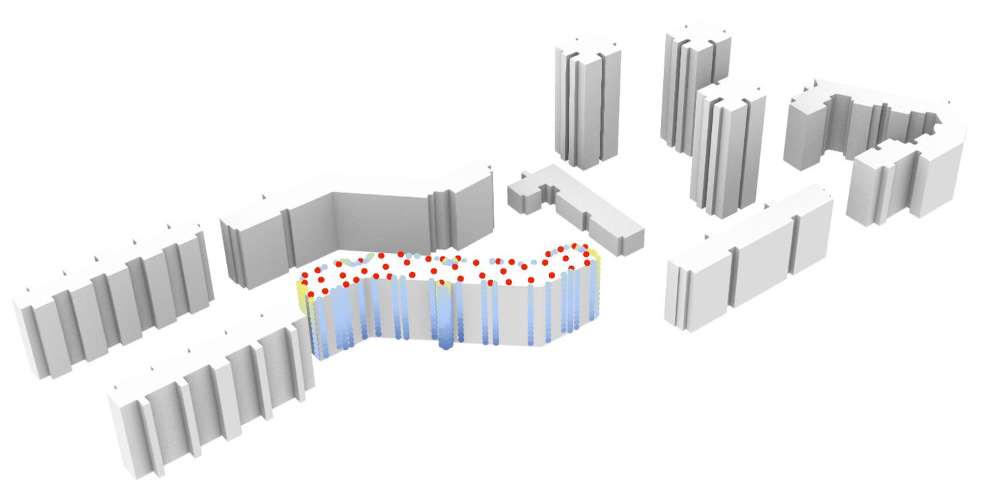
Fig.cea-v-01-04 visualises the building envelopes together with the CEA sensors.

How-to-use-it?

You should be seeing your own visualised results now, if you have followed and successfully executed the four steps presented above. However, how is this useful other than visually and three-dimensionally presenting the solar insolation on each area of the building envelope?

The figure below presents an idea of how such a presentation aids the architectural and urban design process of building-integreated photovoltaics (BIPV). We will discuss the details of this process in the BIPV Design Module. You can click here and proceed to CEA Lesson [cea-b-01].

Questions?

Encountering difficulties or having questions above the processed above? Proceed to the CEA Forum to post your questions. Your questions may be universal and can benefit other CEA users. Please include the Lesson Code [cea-v-01] when posting your question.