
Grasshopper-CEA Part 5: Estimate solar energy potential using CEA in Rhino 6
On the basis of the previous one, in this blog, I am going to introduce how to estimate solar energy potential using CEA functions for your building geometries. I use photovoltaic panels as an example, while CEA is able to perform simulations for other types of solar technologies, such as solar thermal and photovoltaic-thermal technologies. Besides, in this post, I will introduce an easy method to iterate simulations when you have multiple scenarios under the same project umbrella.
Preparation
Before we start, please make sure all the scenarios are stored in the required CEA-file format. See my previous blog for instructions on how to do so with your Grasshopper geometries. The following figure presents the example project under path “D:\ZS\B\800“, which contains 18 scenarios.

CEA photovoltaic panels
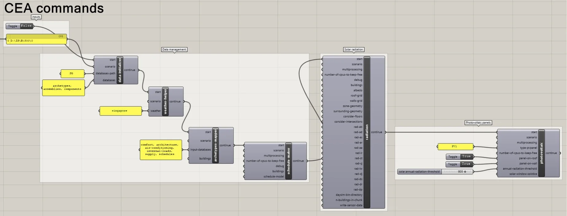
The following figure presents the settings for CEA simulations for photovoltaic panels for the scenario under path “D:\ZS\B\800\1“. Similar to CEA energy demand simulations, the Data management section completes all the missing data. You can always use your own database as the inputs instead of using the CEA defaults. You can also customize the inputs for radiation and energy demand components the same way as you use the CEA dashboards. CEA simulations for photovoltaic panels also require running the radiation command in advance.
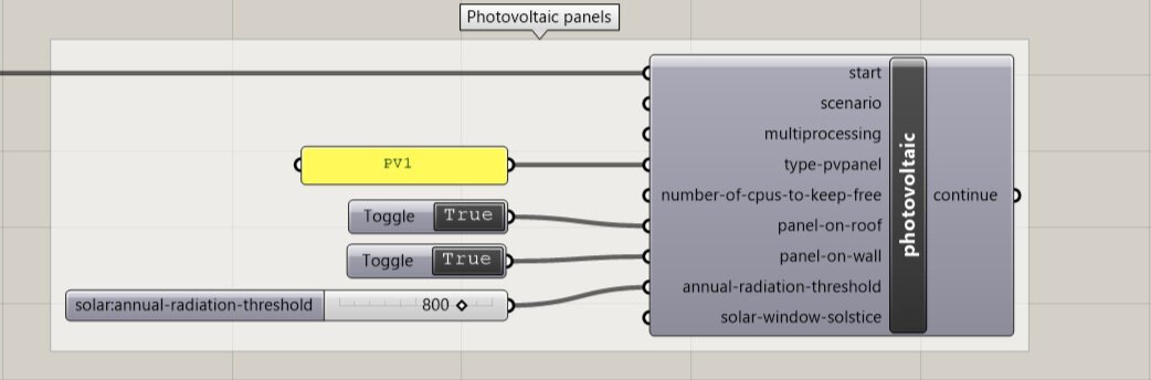
Let’s take a closer look at the settings for the photovoltaic component in the following figure.
In the CEA database, there are three types of photovoltaic panels (“type-pvpanel“). In the example, I select “PV1“. For more details about the attributes of these photovoltaic panels, please check the CEA database under path “C:\Users\Admin\Documents\GitHub\CityEnergyAnalyst\cea\databases\SG\systems\supply_systems.xls“.
The boolean toggles decide whether the photovoltaic are allowed on the building roofs (“panel-on-roof“) or facades (“panel-on-wall“).
In the example, the “annual-radiation-threshold“ for photovoltaic installations is set at 800 kWh/m2/year, which is based on rules-of-thumb and some literature studies. One of our recent studies indicates the threshold can be set at 400 kWh/m2/year. Please find more details in the relevant publication.
The input “solar-window-solstice“ is relevant for the spacing between photovoltaic panels. The default setting is 4 (hours). Please find more details here.
The following figure presents the CEA component of “solar-collector“ and “photovoltaic-thermal“. You can try them out.
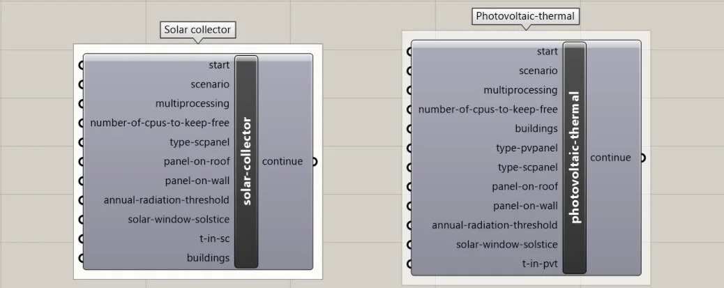
three technologies.PNG
Batch processing
Don’t forget we have 18 scenarios to run for this project. While each project may take hours to complete, you may want to set up an automated processing for the simulations of these 18 scenarios. The following figure presents an easy set-up for iterating simulations using the Grasshopper-Loop plug-in (by Chuyun0316). This set-up gives an “exit” from the loop after the 18 CEA simulations. Of course, there are other ways of achieving automated simulations for multiple scenarios. Please feel free to share your way with us in the comment section below.

Summary
In this post, I introduced how to estimate the solar energy potential using CEA in Rhino 6 with given geometries. The following figure presents the district simulated in Scenario 2. It is generated by a tool called the Urban Block Generator, which I mentioned in my previous blog.

Next
In the next blog, I am going to introduce how the Urban Block Generator can help you populate a district like the one above using block typologies, which I promised last time. Besides estimating the solar energy potential, you can use the generated urban geometries for other design metrics. Should you have any questions, please write them down in the comment section below.
Thanks and keep healthy!