Grasshopper-CEA Part 4: Energy demand forecast using CEA in Rhino 6

How is everything going? We hope everyone is safe and healthy.

While working from home, we have upgraded the interface of CEA for Grasshopper in Rhino 6. In this post, I am going to introduce how to export your Grasshopper geometries to CEA files and perform CEA energy demand simulation in Grasshopper in one workflow. You may ignore the previous version for Rhino 5, which I introduced in the blog titled “Grasshopper-CEA Part 2”. We have stopped maintaining this older version.

The three-step workflow includes installation, CEA-file-making, and CEA energy demand simulation.

The installation

Please follow the next steps for the installation of the CEA interface for Grasshopper/Rhino 6.

1. Make sure you have CityEnergyAnalyst v3.2.0 installed to the default directory

2. Visit here.

3. Download cea-grasshopper.ghpy

4. Copy the file cea-grasshopper.ghpyto the Grasshopper Libraries folder “%APPDATA%\Roaming\Grasshopper\Libraries”

5. you can find the CEA interface under the Tab City Energy Analyst. Different from the older CEA interface, this version has each CEA functions as a stand-alone component. The CEA tab for Grasshopper looks like this:

The CEA tab for Grasshopper.

The CEA-file-making

The inputs for CEA simulations need to follow the CEA-file format. As you may know, the Data management functions help you complete the missing data of your inputs using the CEA database. However, the followings are basic:

• zone.shp It includes the target polygons for simulations. It needs to be stored in “…\scenario-name\inputs\building-geometry\zone.shp“. Its attribute table follows this format:

zone_dbf.PNG

• surroundings.shpIt includes the polygons that surround the zone.shp as the contexts. It needs to be stored in “…\scenario-name\inputs\building-geometry\sorroundings.shp“.Its attribute table follows the same format as zone.shp.

• streets.shpIt includes the polylines of the street centerlines in the district.It is used for thermal network piping layout design, but not necessary for energy demand simulations.Its attribute table contains the information on the length of each polyline.

• terrain.tifIt includes the terrain elevation information.It needs to be stored in “…\scenario-name\inputs\topography\terrain.tif“.

• typology.dbfIt includes the information on each building’s year of construction, standard of construction, and land use mix.It needs to be stored in “…\scenario-name\inputs\building-properties\typology.dbf”.It follows this format:

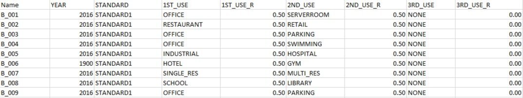
typology_dbf.jpg

To export the grasshopper geometries to the CEA-file format, I use the GHSHP component. Please see my previous blog about the installation and the uses of GHSHP. The following three figures present how the zone.shp, surroundings.shp, and streets.shp are created from the Grasshopper geometries. The exported shapefiles are missing the information geographic coordinate systems. Please download it here and rename it as zone, surroundings, and streets in the building-geometry and the networks folders.

An example of exporting zone.shp

An example of exporting surroundings.shp

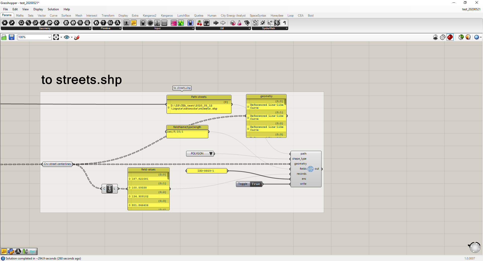
An example of exporting streets.shp

CEA has a “dbf-to-excel-dbf“ function. It can help you convert the typology table following the required format from excel file to dbf file. The following figure presents the settings for using this CEA function.

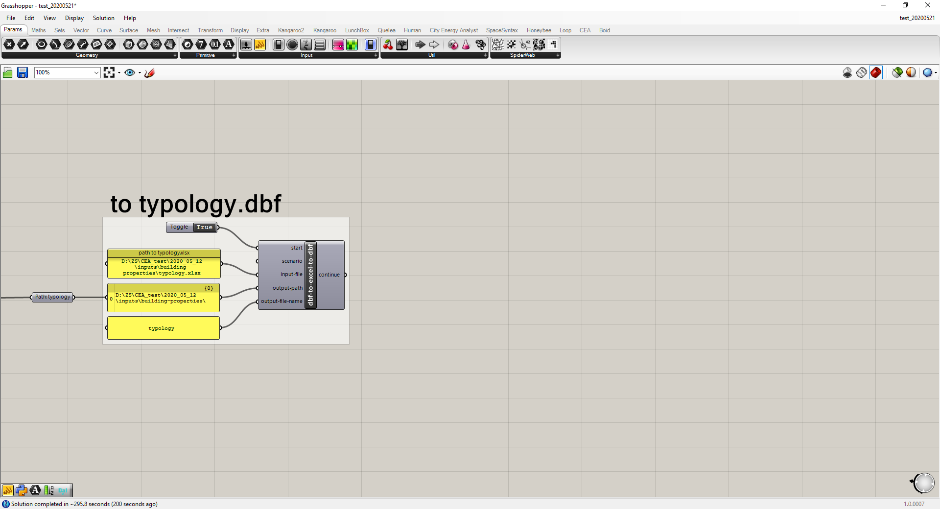
An example of exporting typology.dbf

CEA energy demand simulation

Now that we have the basic CEA files in the right order. They are supposed to be stored in the following path following the required format:

“…\scenario-name\inputs\building-geometry\zone.shp”

“…\scenario-name\inputs\building-geometry\zone.prj”

“…\scenario-name\inputs\building-geometry\surroundings.shp”

“…\scenario-name\inputs\building-geometry\surroundings.prj”

“…\scenario-name\inputs\networks\streets.shp”

“…\scenario-name\inputs\networks\streets.prj”

“…\scenario-name\inputs\topography\terrain.tif'“

“…\scenario-name\inputs\building-properties\typology.dbf'“

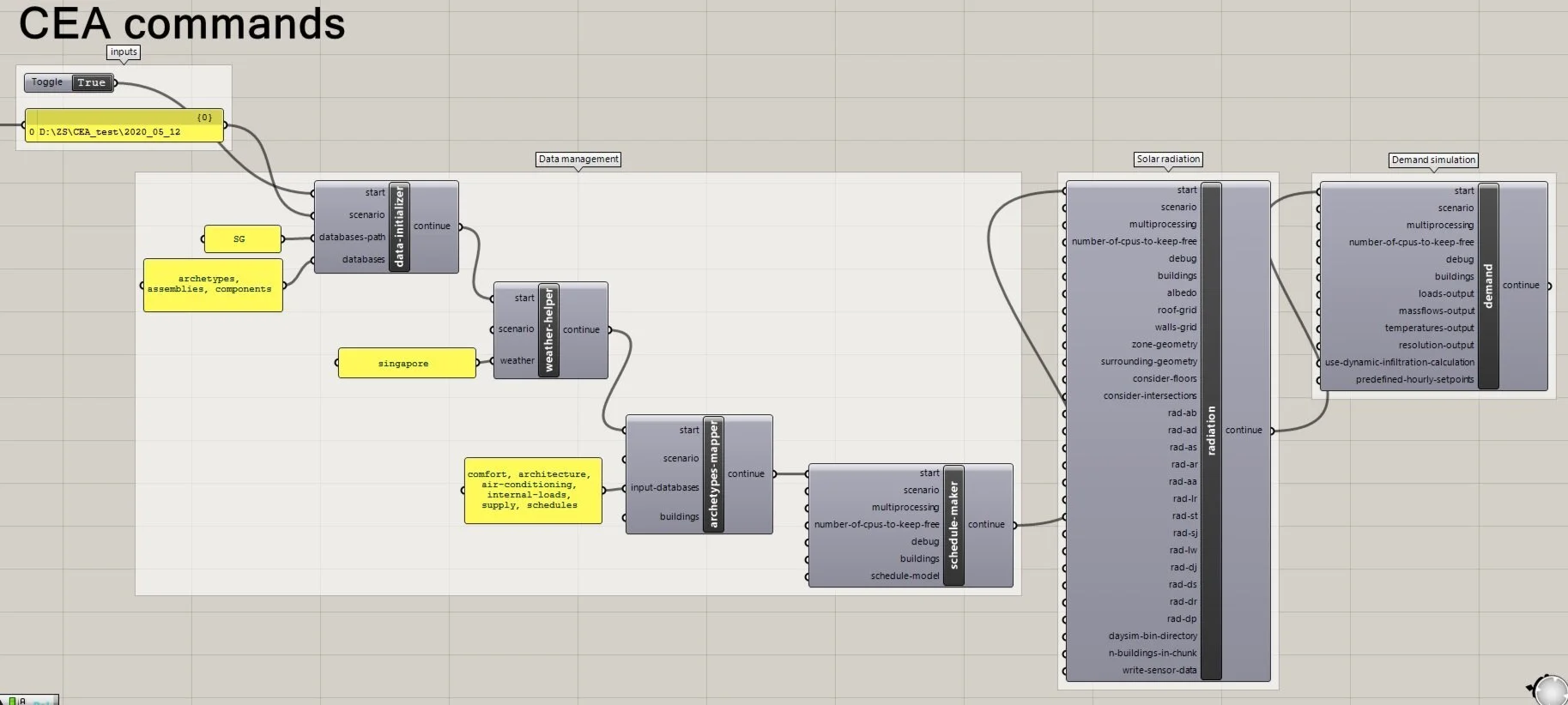
The following figure presents the settings for CEA energy demand simulation using the CEA files we have just prepared. The Data management section completes all the missing data. Of course, you can always use your own database as the inputs instead of using the CEA defaults. You can also customize the inputs for radiation and energy demand components the same way as you use the CEA dashboards.

Summary

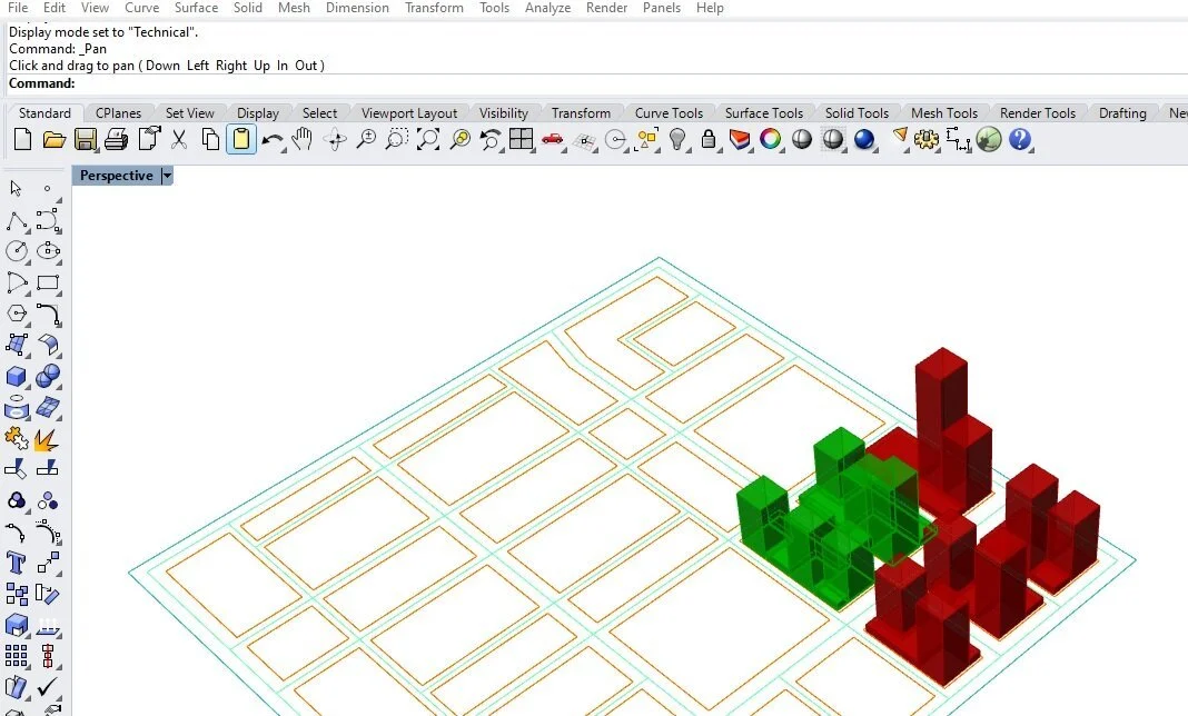
In this post, I introduced how to export your Grasshopper geometries to CEA files and perform CEA energy demand simulation in Grasshopper in one workflow. For your reference, please find the example I used above here. As you may notice, in the CEA-file-making, I manually entered all the data while you can always seek to make these data concerning the zone.shp, surroundings.shp, streets.shp, and typology.dbf parametric for your research. The following figure presents the 3D illustrations of the zone (green), surroundings (red), and streets (aquamarine). It is generated by a tool called the Urban Block Generator.

Next

In the next blog, I am going to introduce how the Urban Block Generator can help you generate building geometries from scratch for CEA simulations and parametric studies. Before I finish, I would like to thank Daren Thomas for building this new CEA interface for Grasshopper/Rhino 6 and Theresa Fink for the tips on GHSHP. Should you have any questions, please write them down in the comment section below.

Thanks and keep healthy!