
Grasshopper-CEA Part 1: Creating input files in .dbf format
In a series of posts, I would like to introduce using the City Energy Analyst (CEA) with Grasshopper. The linkage between the two tools is named as GTC, short for Grasshopper-to-CEA. GTC enables the users to conduct automated iterations with CEA and the parametric model in Grasshopper, serving purposes like optimization or sensitivity analysis. GTC has two main functions. One is that it functions as a parser, which converts the format of the geometries generated in Grasshopper to the CEA format. The other one is that it calls CEA to perform the simulations off the platform of Grasshopper. As the introductory post, this post introduces the installation of GTC and demonstrates creating input files in .dbf format with GTC.
Installation of GTC on Windows
The installation script was downloaded to your computer when you installed CEA. To install GTC, simply follow the four steps as follows.
1. Make sure Rhino5 and Grasshopper v0.9.0076 are successfully installed.
2. Launch the CEA Console from the start menu.
3. Type cea install-grasshopper and press ENTER.
Repeat Step 2 through 3 every time you update CEA with Github.
4. Launch Rhino 5 and Grasshopper and you should see CEA on the component tabs. The CEA component looks like this and it is normal it displays as “in-error“ before a successful execution.
Following is a short animation displaying how to make the installation.
The process of installing GTC on your computer after you successfully installed CEA.
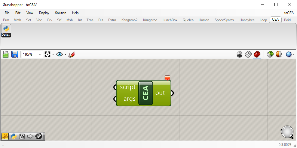
The CEA component in Grasshopper
Creating .dbf files
Both age.dbf and occupancy.dbf are two prerequisites for CEA simulations. They follow their own strict template. Example files of both age.dbf and occupancy.dbf are shown as follows. Make excel tables following the exact same template as in the figure below.
In the age table, the “built” column indicates the year of built for the building, while the rest of the columns indicate the year of renovation for that particular building component. If they are not ever renovated, keep the corresponding cells as “0“. For example, in the figure, Building “B001” was built in the Year of 2018, and none of the building components was renovated since the construction.
In the occupancy table, the fraction of each land use (function) shall add up to 1. For example, in the figure, Building “B001“ has only three functions: office (30%), retail (10%), and multi-family residential (60%). Keep the rest as “0“.
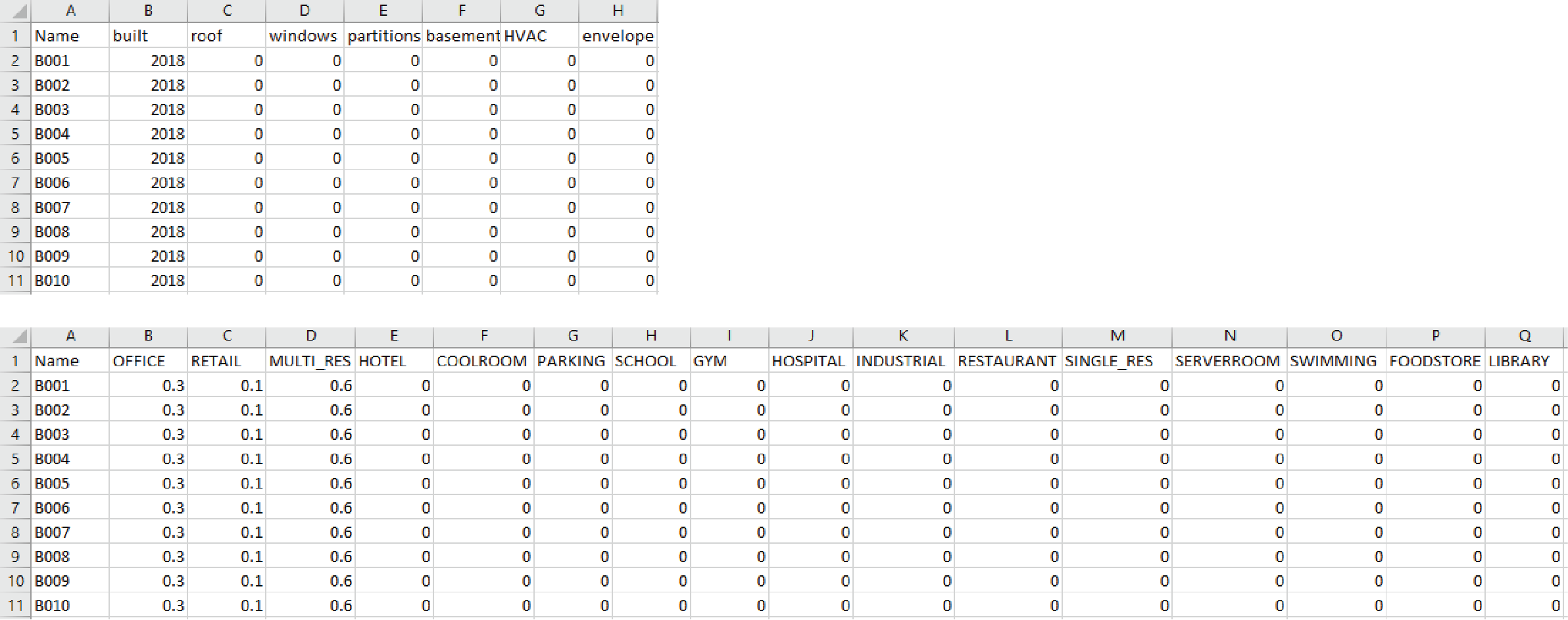
Example age (up) and occupancy (down) files
The next figure illustrates how to set up the two inputs for the CEA component in Grasshopper to convert the excel files you have to the .dbf format required for CEA simulations. The processing of such conversions should be really fast. After a successful execution, the CEA component will turn to “grey“ from “red“ and you can see the .dbf files created in your output folder. Please note that the input and output-path does not necessarily to follow the format of CEA files.
The steps are as follows.
1. Connect panel “dbf-to-excel-to-dbf“ to the CEA component by “script“
2. Connect the panel containing the input and output information to the CEA component by “args“
input-file=the path of the input excel file
output-file-name=the name of the output .dbf file without the extension
output-path=the path of the enclosing folder for the output .dbf file
3. Check the converted .dbf file in your target folder
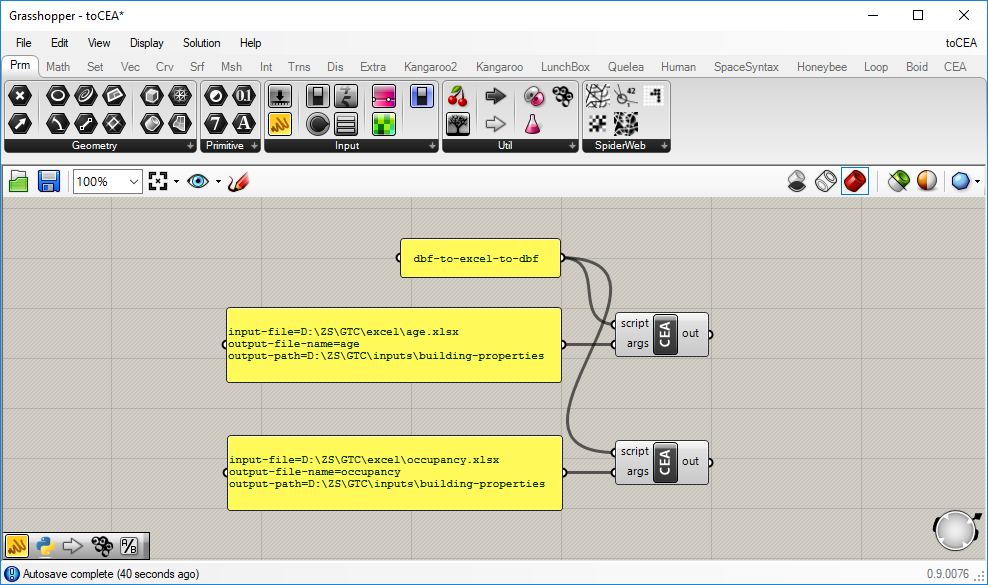
Set-ups in grasshopper for producing age.dbf and occupancy.dbf
Now, you should have the required .dbf format for both age and occupancy in CEA simulations.
Give it a try and comment below to let me know how it goes.
Next
In the coming posts, I am going to introduce how to run CEA commands in Grasshopper.

Dr. Zhongming Shi
Sep 8, 2018
Sep 8, 2018
Researcher at the Singapore-ETH Centre of the ETH Zurich
E-mail | ResearchGate | LinkedIn | GoogleScholar | Github
Sep 8, 2018
If you like this post, please give it a like or share it. Thanks!