GUIDEBOOK · CEA v4.0
Final Energy
Final Energy
Overview
Calculates the final energy consumed by each building and district plant under a specific supply configuration (what-if scenario). Final energy is what the energy system actually consumes from carriers (grid electricity, natural gas, oil, coal, wood) to meet the building’s energy demand.
What It Calculates
For each building:
- Energy carrier consumption per service (heating, cooling, DHW, electricity)
- Conversion losses based on technology efficiency
- Booster energy for district-connected buildings
For each district plant (DH/DC):
- Primary and tertiary conversion energy
- Network pumping electricity
Prerequisites
- Energy Demand Part 2 completed
- Solar Radiation completed (if PV/PVT/SC are configured)
- Thermal Network Part 1 + Part 2 completed (if district network scenarios are used)
- Building supply settings configured (Building Properties > Supply tab)
Key Parameters
| Parameter | Description |
|---|---|
| What-if name | Name for this supply configuration scenario |
| Network name | Which thermal network layout to use (if applicable) |
| Supply type (heating/cooling/DHW) | Assembly codes for building and/or district scale |
| Overwrite supply settings | True to use what-if mode instead of production mode |
| Connected buildings | Override which buildings connect to the network |
How to Use
-
Configure supply systems in Building Properties > Supply tab:
- Set scale (BUILDING or DISTRICT) per service per building
- Assign conversion technologies and carriers
-
Run Final Energy:
- Navigate to Life Cycle Analysis
- Select Final Energy
- Enter a what-if scenario name
- Select network layout (if buildings use district services)
- Click Run
-
Processing time: 1-5 minutes for typical districts
Output Files
All outputs are stored under {scenario}/outputs/data/analysis/{what-if-name}/final-energy/:
| File | Description |
|---|---|
configuration.json | Full supply configuration (buildings + plants). Used by all downstream features. |
final_energy_buildings.csv | Annual summary per entity (buildings + plants) |
{building_name}.csv | 8,760-row hourly energy by carrier per building |
{plant_name}.csv | 8,760-row hourly energy by carrier per plant |
Understanding Results
- Building-scale systems: Final energy = demand / efficiency
- District-connected buildings: Show DH/DC as their carrier; actual fuel consumption is at the plant level
- Plants: Appear as separate rows with
type=plant; their carrier consumption covers all connected buildings plus network losses and pumping configuration.json: Stores the complete supply configuration and is the sole source of truth for emissions, costs, and heat rejection
Solar-thermal DHW dispatch (SC primary)
When a hot-water assembly uses a flat-plate (SC1) or evacuated-tube
(SC2) solar collector as the primary component, the Final Energy
feature runs an hourly tank-dispatch model instead of the usual “fuel =
demand / efficiency” shortcut.
What the model does
- Reads
Q_SC_gen_kWhfrom the SC potential file, summing only the(surface, panel_type)pairs configured for this building (not the full panel-type aggregate — see Solar Collectors output files). - Charges a single-node fully-mixed tank, sized at 50 L per m² of SC aperture and initialised at the hour-0 cold-mains inlet temperature.
- Serves DHW demand from the tank through a thermostatic mixing valve
(setpoint 60 °C, the standard CEA
TWW_SETPOINT). When the tank is below setpoint, the secondary component (BO/HP) tops up the gap. - Applies a Newton-style standing loss toward 20 °C ambient at 2%/hr.
- Dumps surplus heat that would push the tank above 105 °C (pressure-relief cap).
Assembly requirements
primary_componentmust be an SC code (SC1orSC2).secondary_componentis required — solar alone cannot cover 24/7 DHW. Must be a boiler (BO*) or heat pump (HP*). The validator rejects assemblies without a backup.- PVT cannot be a DHW primary. Its ~35 °C operating temperature is below the DHW setpoint and would need a stratified tank model to credit meaningfully. Configure an SC primary instead; PVT continues to offset space-heating emissions via the legacy path.
Output columns (per-building B####.csv)
| Column | Meaning |
|---|---|
Qww_sys_SOLAR_kWh | Hourly solar-delivered share of DHW (zero-emission carrier) |
Qww_sys_{backup}_kWh | Hourly backup-carrier share (e.g. Qww_sys_GRID_kWh for an electric BO5 backup). Equals served_by_backup_kwh / backup_efficiency. |
Qww_sys_SOLAR_dumped_kWh | Diagnostic: hourly heat discarded at the T_MAX=105 °C cap. Non-zero values flag an oversized SC for the DHW load. |
E_sys_GRID_kWh | Includes SC pump parasitic (2% of delivered solar, added to the grid-electricity stream) |
The carrier-aggregation pipelines (summary CSV, emissions, costs,
visualisation) filter out *_dumped_kWh so it doesn’t inflate totals.
Known caveats
- Oversizing is not a bug; it’s visible. If
area_SC_m2is much larger than DHW demand justifies, the tank becomes large enough that standing losses dominate delivered heat. CheckQww_sys_SOLAR_dumped_kWhand the gapQ_SC_gen − Qww_sys_SOLAR_kWh − Qww_sys_SOLAR_dumped_kWh(standing loss) to diagnose. - Self-consistent T_cold bias: The cold-mains inlet series used by
both the demand side (
Qww_sys_kWh) and the dispatch side comes fromcea.demand.hotwater_loads.calc_water_temperature, which has a pre-existing units bug (uses hours where the Kusuda 1965 model expects seconds) that collapses the series to a constant. Real-world solar fractions in temperate climates are likely ~10% higher than the model reports. Tracked separately from this feature.
Troubleshooting
| Issue | Solution |
|---|---|
| ”Multiple district heating assembly types detected” | All district buildings must use the same assembly. Provide only one district assembly per service. |
| ”District substation file not found” | Run thermal-network Part 2 before final-energy for scenarios with district connections. |
| ”Component not found” | Check that ASSEMBLIES references valid COMPONENTS codes in the database. |
Plot - Final Energy
Overview
Creates bar charts of final energy consumption by carrier for buildings and plants.
What It Shows
- Stacked bars per building showing carrier breakdown (Grid, Natural Gas, Oil, Coal, Wood)
- Plant entities shown with
-DHor-DCsuffix - Multiple what-if scenarios can be compared side by side
Key Parameters
| Parameter | Description | Options |
|---|---|---|
| What-if name | Which scenario(s) to plot | Multi-select from available |
| Y metric | Which carrier(s) to show | Grid electricity, Natural gas, Oil, Coal, Wood |
| Y unit | Energy unit | MWh, kWh, Wh |
| Normalise by | Normalisation | None, Gross floor area, Conditioned floor area |
| X axis | View type | By building, by month, by season, district hourly, etc. |
| Include | Entity filter | Buildings, Plants, or both |
Examples
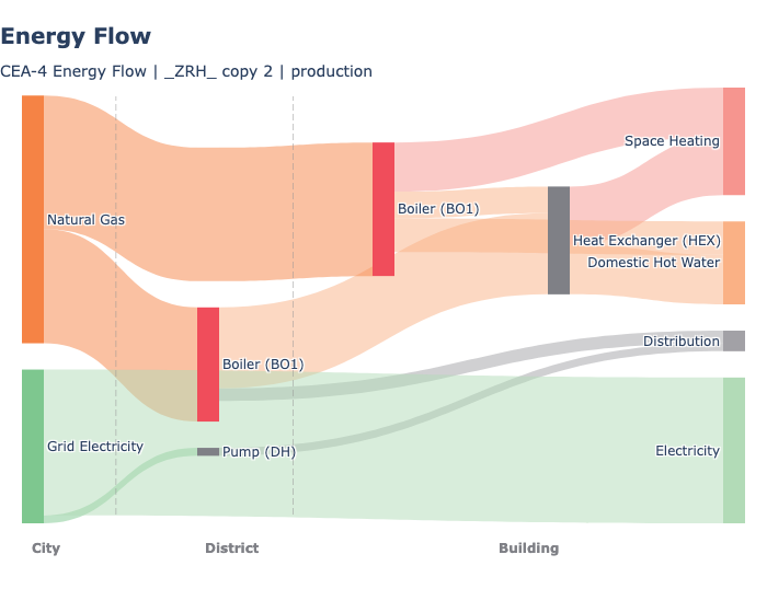
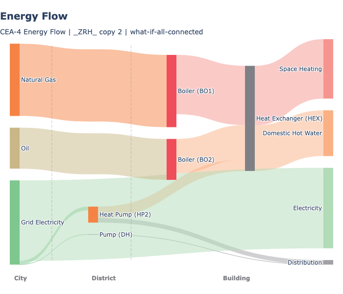
Two what-if scenarios (Config 1 and Config 2) showing different supply configurations for the same district:
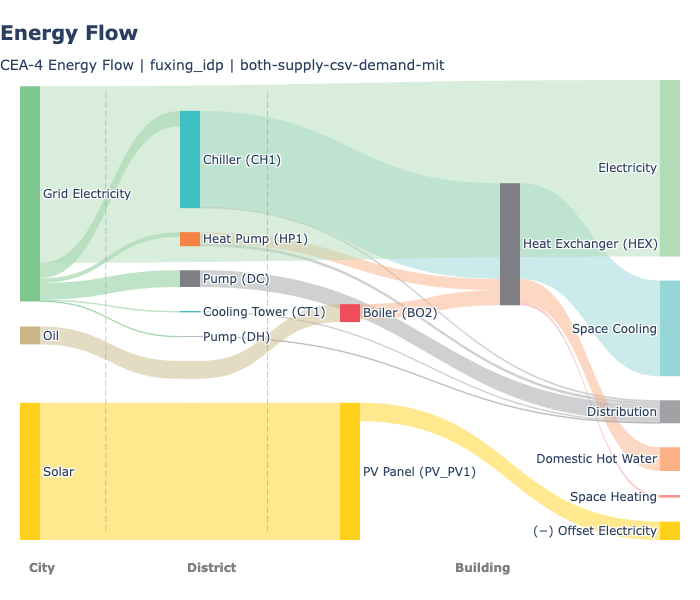
A more complex scenario with district heating, district cooling, and solar:
Load duration curve showing the same component (BO1) across district plant, standalone buildings, and boosters:
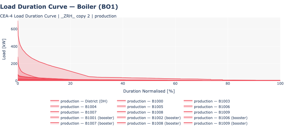
Chart Interpretation
- Energy flow sankey shows carrier flows from city-level sources through district and building equipment to end-use services
- Load duration curve shows the hourly load profile of a component sorted by magnitude, useful for equipment sizing and utilisation analysis
Related Features
- Emissions - Uses final energy to calculate operational emissions
- System Costs - Uses final energy to calculate operational costs
- Heat Rejection - Uses final energy to calculate waste heat
<- Back: Life Cycle Analysis | Back to Index | Next: Emissions ->
Source: view raw on GitHub ↗